Supplement 2: Derivation of tidal force in the accelerated frame

In order to show that tidal force appears when the earth is merely subjected to gravity from a celestial body, let us start from the equations of motion and derive the tidal force that appears on the earth. As a celestial body, we shall consider only the moon.

First, let us write the equations of motion in the inertial frame of reference. Let P be a point on the earth, E be the center of the earth, and L be the center of the moon. In addition, let the mass of the earth be \( {M} \), the mass of the moon be \( {m} \), and the gravitational constant be \( {G} \). Then, the equation of motion for the point P is as follows. The first term on the right side is the gravity of the earth, and the second term is the gravity of the moon.

\[ \frac{{{{\text{d}}^2}{{\boldsymbol{r}}_{\text{P}}}}}{{{\text{d}}{t^2}}} = - \frac{{GM}}{{{{\left| {{{\boldsymbol{r}}_{\text{P}}} - {{\boldsymbol{r}}_{\text{E}}}} \right|}^3}}}({{\boldsymbol{r}}_{\text{P}}} - {{\boldsymbol{r}}_{\text{E}}}) - \frac{{Gm}}{{{{\left| {{{\boldsymbol{r}}_{\text{P}}} - {{\boldsymbol{r}}_{\text{L}}}} \right|}^3}}}({{\boldsymbol{r}}_{\text{P}}} - {{\boldsymbol{r}}_{\text{L}}}) . \tag{1} \]

On the other hand, the equation of motion for the earth center E is as follows. The right side is the gravity of the moon.

\[ \frac{{{{\text{d}}^2}{{\boldsymbol{r}}_{\text{E}}}}}{{{\text{d}}{t^2}}} = - \frac{{Gm}}{{{{\left| {{{\boldsymbol{r}}_{\text{E}}} - {{\boldsymbol{r}}_{\text{L}}}} \right|}^3}}}({{\boldsymbol{r}}_{\text{E}}} - {{\boldsymbol{r}}_{\text{L}}}) . \tag{2} \]

Subtracting Eq. (2) from Eq. (1), we obtain the equation of motion of the point P seen from the center E of the accelerating earth:

\[ \frac{{{{\text{d}}^2}\left( {{{\boldsymbol{r}}_{\text{P}}} - {{\boldsymbol{r}}_{\text{E}}}} \right)}}{{{\text{d}}{t^2}}} = - \frac{{GM}}{{{{\left| {{{\boldsymbol{r}}_{\text{P}}} - {{\boldsymbol{r}}_{\text{E}}}} \right|}^3}}}({{\boldsymbol{r}}_{\text{P}}} - {{\boldsymbol{r}}_{\text{E}}}) - \frac{{Gm}}{{{{\left| {{{\boldsymbol{r}}_{\text{P}}} - {{\boldsymbol{r}}_{\text{L}}}} \right|}^3}}}({{\boldsymbol{r}}_{\text{P}}} - {{\boldsymbol{r}}_{\text{L}}}) + \frac{{Gm}}{{{{\left| {{{\boldsymbol{r}}_{\text{E}}} - {{\boldsymbol{r}}_{\text{L}}}} \right|}^3}}}({{\boldsymbol{r}}_{\text{E}}} - {{\boldsymbol{r}}_{\text{L}}}) . \tag{3} \]

To simplify the equation, let \({\boldsymbol{r}}\) be the position of point P seen from the earth center E and \({\boldsymbol{a}}\) be the position of the moon L seen from the earth center E. Then we can write \({{\boldsymbol{r}}_{\text{P}}} - {{\boldsymbol{r}}_{\text{E}}} = {\boldsymbol{r}}\), \({{\boldsymbol{r}}_{\text{P}}} - {{\boldsymbol{r}}_{\text{L}}} = {\boldsymbol{r}} - {\boldsymbol{a}}\), \({{\boldsymbol{r}}_{\text{E}}} - {{\boldsymbol{r}}_{\text{L}}} = -{\boldsymbol{a}}\), and Eq. (3) becomes as simple as Eq. (4). On the right side of Eq. (4), the first term is the gravity of the earth, the second term is the gravity of the moon, and the third term is the translational inertial force.

\[ \frac{{{{\text{d}}^2}{\boldsymbol{r}}}}{{{\text{d}}{t^2}}} = - \frac{{GM}}{{{r^3}}}{\boldsymbol{r}} - \frac{{Gm}}{{{{\left| {{\boldsymbol{r}} - {\boldsymbol{a}}} \right|}^3}}}({\boldsymbol{r}} - {\boldsymbol{a}}) - \frac{{Gm}}{{{a^3}}}{\boldsymbol{a}} . \tag{4} \]

In order to obtain the expression for the potential, the right-hand side of Eq. (4) should be written using the differential operator as follows:

\[ \frac{{{{\text{d}}^2}{\boldsymbol{r}}}}{{{\text{d}}{t^2}}} = - \frac{\partial }{\partial {\boldsymbol{r}}} \left( { - \frac{{GM}}{r} - \frac{{Gm}}{{\sqrt {{{\left( {{\boldsymbol{r}} - {\boldsymbol{a}}} \right)}^2}} }} + \frac{{Gm}}{{{a^3}}}{\boldsymbol{a}} \cdot {\boldsymbol{r}}} \right) . \tag{5} \]

The parentheses on the right side of Eq. (5) is the potential seen from the accelerating earth. Let \(V'\) denote this potential. Using \(x\), \(y\), and \(z\), this potential can be expressed by the following equation, where \(x\) is in the direction of \(\boldsymbol{a}\), or the direction of the moon seen from the earth.

\[ V' = - \frac{{GM}}{{\sqrt {{x^2} + {y^2} + {z^2}} }} - \frac{{Gm}}{{\sqrt {{{(x - a)}^2} + {y^2} + {z^2}} }} + \frac{{Gm}}{{{a^2}}}x. \tag{6} \]

Assuming that \(x\), \(y\), and \(z\) are sufficiently small compared to \(a\), the second term in Eq. (6) can be approximated by an expansion up to the second order term as in Eq. (7). On the right-hand side of Eq. (7), the second term represents the gravity of the moon at the earth center, and the third term represents the deviation of gravity from that at the earth center, i.e. the tidal force.

\[ - \frac{{Gm}}{{\sqrt {{{(x - a)}^2} + {y^2} + {z^2}} }} \approx - \frac{{Gm}}{a} - \frac{{Gm}}{{{a^2}}}x - \frac{{Gm}}{{{a^3}}}({x^2} - \tfrac{1}{2}{y^2} - \tfrac{1}{2}{z^2}) . \tag{7} \]

Substituting Eq. (7) into the second term of Eq (6), we can approximate the potential seen in the accelerated frame by the following equation, excluding the constant term:

\[ V' \approx - \frac{{GM}}{{\sqrt {{x^2} + {y^2} + {z^2}} }} - \frac{{Gm}}{{{a^3}}}\left( {{x^2} - \tfrac{1}{2}{y^2} - \tfrac{1}{2}{z^2}} \right) . \tag{8} \]

Consequently, the only forces that can be seen from the accelerating earth are the gravitational force of the earth in the first term and the tidal force in the second term. This equation is Eq. (5) on the main page of this article.

Let us derive the tidal potential from Eq. (4) using a different method. In Eq. (4), we can approximate a part of the term as follows:

\[ \begin{align} \frac{1}{{{{\left| {{\boldsymbol{r}} - {\boldsymbol{a}}} \right|}^3}}} &= {\left[ {{{({\boldsymbol{r}} - {\boldsymbol{a}})}^2}} \right]^{ - 3/2}} \\ &= \frac{1}{{{a^3}}}{\left( {1 - \frac{{2{\boldsymbol{a}} \cdot {\boldsymbol{r}}}}{{{a^2}}} + \frac{{{r^2}}}{{{a^2}}}} \right)^{ - 3/2}} \\ &\approx \frac{1}{{{a^3}}} + \frac{{3{\boldsymbol{a}} \cdot {\boldsymbol{r}}}}{{{a^5}}} . \tag{9} \\ \end{align} \]

Substituting this relation into Eq. (4) and ignoring the second order terms in \(r\), we can rewrite Eq. (4) as

\[ \begin{align} \frac{{{{\text{d}}^2}{\boldsymbol{r}}}}{{{\text{d}}{t^2}}} &\approx - \frac{{GM}}{{{r^3}}}{\boldsymbol{r}} - \frac{{Gm}}{{{a^3}}}({\boldsymbol{r}} - {\boldsymbol{a}}) + \frac{{3Gm({\boldsymbol{a}} \cdot {\boldsymbol{r}}){\boldsymbol{a}}}}{{{a^5}}} - \frac{{Gm}}{{{a^3}}}{\boldsymbol{a}} \\ &= - \frac{{GM}}{{{r^3}}}{\boldsymbol{r}} + \frac{{Gm}}{{{a^3}}}\left[ {\frac{{3({\boldsymbol{a}} \cdot {\boldsymbol{r}}){\boldsymbol{a}}}}{{{a^2}}} - {\boldsymbol{r}}} \right]. \tag{10} \\ \end{align} \]

\[ \frac{{{{\text{d}}^2}{\boldsymbol{r}}}}{{{\text{d}}{t^2}}} = - \frac{{\partial V'}}{{\partial {\boldsymbol{r}}}}. \tag{11} \]

\[ V' \approx - \frac{{GM}}{r} - \frac{{Gm}}{{2{a^3}}}\left[ {\frac{{3{{({\boldsymbol{a}} \cdot {\boldsymbol{r}})}^2}}}{{{a^2}}} - {r^2}} \right]. \tag{12} \]

The first term is the gravity due to the earth and the second term is the tidal force due to the moon. Using \(x\), \(y\), and \(z\), this potential can be expressed by the same equation as Eq. (8), where \(x\) is in the direction of \(\boldsymbol{a}\), or the direction of the moon seen from the earth.

\[ V' \approx - \frac{{GM}}{{\sqrt {{x^2} + {y^2} + {z^2}} }} - \frac{{Gm}}{{{a^3}}}\left( {{x^2} - \tfrac{1}{2}{y^2} - \tfrac{1}{2}{z^2}} \right) . \]

For reference, if we put \(x = r\sin \theta \cos \varphi\), \(y = r\sin \theta \sin \varphi\), \(z = r\cos \theta\), the potential \(V'\) can be expressed in the spherical coordinates:

\[ V' \approx - \frac{GM}{r} - \frac{{Gm}}{{2{a^3}}}{r^2}(3{\sin ^2}\theta {\cos ^2}\varphi - 1) . \tag{13} \]

Let \( R \) be the radius of the earth in the absence of the tidal force and \( \zeta \) be the vertical displacement of the equipotential surface due to the tidal force. If the sea water movement is fast enough to reach equilibrium, and if the potential change due to the deformation of the earth and the movement of the sea water is negligible, then the sea level will rise by \( \zeta \), following the equipotential surface. Now, substituting \( r=R+\zeta \) to Eq. (12) and assuming that \( \zeta \) is sufficiently small compared to \( R \), we obtain

\[ V' \approx - \frac{{GM}}{R}\left( {1 - \frac{\zeta}{R}} \right) - \frac{{Gm}}{{2{a^3}}}\left[ {\frac{{3{{\left( {{\boldsymbol{a}} \cdot {\boldsymbol{R}}} \right)}^2}}}{{{a^2}}} - {R^2}} \right]. \tag{14} \]

Since this is equal to \( - GM/R \), the equation for the rise of the sea level of equilibrium tide becomes

\[ \zeta = \frac{{m{R^4}}}{{2M{a^3}}}\left[ {\frac{{3{{\left( {{\boldsymbol{a}} \cdot {\boldsymbol{R}}} \right)}^2}}}{{{a^2}{R^2}}} - 1} \right]. \tag{15} \]

Fig. 3. Coordinate system fixed to the rotating earth. The angle \( \lambda \) is the latitude of the observation point, \( \delta \) is the declination of the moon, and \( H \) is the hour angle of the moon.

In Eq. (13) we considered a coordinate system based on the direction of the moon at a certain moment. Here we will use the coordinate system fixed to the earth. In this case, the direction of the moon is generally off the equatorial plane. Let \( \lambda \) be the latitude of the observation point, \( \delta \) be the declination of the moon, and \( H \) be the hour angle (the angle measured westward from the meridian of the observation point) of the moon (see Fig. 3). If \( x \) is the equatorial direction on the meridian of the observation point, the position of the observation point is given by \( {\boldsymbol{R}} = (R\cos \lambda ,\,\, 0,\,\,R\sin \lambda ) \), and the position of the moon is \( {\boldsymbol{a}} = (a\cos \delta \cos H,\, - a\cos \delta \sin H,\,\,a\sin \delta ) \). Substituting these vectors into equation (15) and arranging the trigonometric functions, we obtain the following equation for the rise of the equipotential surface:

\[ \zeta = \frac{{3m{R^4}}}{{4M{a^3}}}\left[ {{{\cos }^2}\lambda {{\cos }^2}\delta \cos 2H + \sin 2\lambda \sin 2\delta \cos H + 3\left( {{{\sin }^2}\lambda - \frac{1}{3}} \right)\left( {{{\sin }^2}\delta - \frac{1}{3}} \right)} \right]. \tag{16} \]

In the above equation, the hour angle \( H \) changes about \( 2\pi \) per day due to the earth's rotation. Therefore, the first term in Eq. (16) represents a semidiurnal tide (a tide with a period of about half a day). The second term is a diurnal tide (a tide with a period of about one day), which appear when the moon's declination \( \delta \) is non-zero. Because of this diurnal tide, if the moon is north of the equator for example, high tides become higher when the moon is above the horizon and lower when the moon is below the horizon in the northern hemisphere. The third term represents the long-period deformation in the polar direction, which changes slowly with a period of about 13.7 days and a period of half a year, due to the variation of the moon's declination \( \delta \) caused by the inclination of the ecliptic from the equatorial plane and the inclination of the lunar orbit from the ecliptic plane (see Fig. 4). If the sea level deforms according to the potential, the rise of the sea level can be described by this equation. However, the actual motion of sea water is much more complicated due to the slow response and the friction of sea water, and the influence of ocean topography and the Coriolis forces.


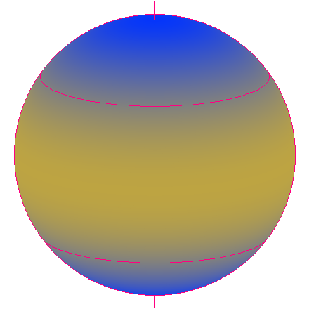(1) semidiurnal tide	(2) diurnal tide	(3) long period tide
Fig. 4. Three types of tides. Click on images (1), (2) to start animations.